Jerry Licun Pages

Week6 Lab -- ggplot做复杂图     (具体Tutor代码)

Decomposing the date：	library(lubridate)
ped_melb.south.bourke <- ped_melb.south.bourke %>%
         mutate(year = year(Date),
         month = month(Date, label = TRUE, abbr = TRUE), 
         wday = wday(Date, label = TRUE, abbr = TRUE, week_start = 1),
         day = day(Date))

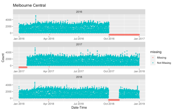
Exploring time gaps：	library(naniar)
ped_melb.south.bourke %>% 
  	filter(Sensor == "Melbourne Central") %>%
  	ggplot(aes(x=Date_Time, y=Count)) + 
  	geom_miss_point(size = 0.7) +
  	facet_wrap(year ~., scales = "free_x", nrow = 3) +
  	labs(title = "Melbourne Central", y = "Count", x = "Date-Time")
 
 
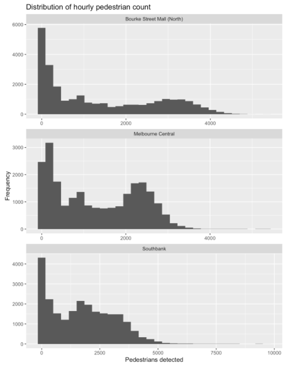
Distribution of count:
ped_melb.south.bourke %>%
  	ggplot(aes(x = Count)) +
  	geom_histogram() +
  	labs(title = "Distribution of hourly pedestrian count", 
       	x = "Pedestrians detected",
       	y = "Frequency") +
  	facet_wrap(~ Sensor, scales = "free", nrow = 3)


Activity 6.2 
运用Pedestrian数据： 做复杂的Histogram图、Line图、Boxplot图